Mesh Processing in Python: Implementing ARAP deformation
Python is a pretty nice language for prototyping and (with numpy and scipy) can be quite fast for numerics but is not great for algorithms with frequent tight loops. One place I run into this frequently is in graphics, particularly applications involving meshes.
Not much can be done if you need to frequently modify mesh structure. Luckily, many algorithms operate on meshes with fixed structure. In this case, expressing algorithms in terms of block operations can be much faster. Actually implementing methods in this way can be tricky though.
To gain more experience in this, I decided to try implementing the As-Rigid-As-Possible Surface Modeling mesh deformation algorithm in Python. This involves solving moderately sized Laplace systems where the right-hand-side involves some non-trivial computation (per-vertex SVDs embedded within evaluation of the Laplace operator). For details on the algorithm, see the link.
As it turns out, the entire implementation ended up being just 99 lines and solves 1600 vertex problems in just under 20ms (more on this later). Full code is available.
Building the Laplace operator
ARAP uses cotangent weights for the Laplace operator in order to be relatively independent of mesh grading. These weights are functions of the angles opposite the edges emanating from each vertex. Building this operator using loops is slow but can be sped up considerably by realizing that every triangle has exactly 3 vertices, 3 angles and 3 edges. Operations can be evaluated on triangles and accumulated to edges.
Here's the Python code for a cotangent Laplace operator:
from typing import *
import numpy as np
import scipy.sparse as sparse
import scipy.sparse.linalg as spla

def build_cotan_laplacian( points: np.ndarray, tris: np.ndarray ):
    a,b,c = (tris[:,0],tris[:,1],tris[:,2])
    A = np.take( points, a, axis=1 )
    B = np.take( points, b, axis=1 )
    C = np.take( points, c, axis=1 )

    eab,ebc,eca = (B-A, C-B, A-C)
    eab = eab/np.linalg.norm(eab,axis=0)[None,:]
    ebc = ebc/np.linalg.norm(ebc,axis=0)[None,:]
    eca = eca/np.linalg.norm(eca,axis=0)[None,:]

    alpha = np.arccos( -np.sum(eca*eab,axis=0) )
    beta  = np.arccos( -np.sum(eab*ebc,axis=0) )
    gamma = np.arccos( -np.sum(ebc*eca,axis=0) )

    wab,wbc,wca = ( 1.0/np.tan(gamma), 1.0/np.tan(alpha), 1.0/np.tan(beta) )
    rows = np.concatenate((   a,   b,   a,   b,   b,   c,   b,   c,   c,   a,   c,   a ), axis=0 )
    cols = np.concatenate((   a,   b,   b,   a,   b,   c,   c,   b,   c,   a,   a,   c ), axis=0 )
    vals = np.concatenate(( wab, wab,-wab,-wab, wbc, wbc,-wbc,-wbc, wca, wca,-wca, -wca), axis=0 )
    L = sparse.coo_matrix((vals,(rows,cols)),shape=(points.shape[1],points.shape[1]), dtype=float).tocsc()
    return L
Inputs are float \(3 \times N_{verts}\) and integer \(N_{tris} \times 3\) arrays for vertices and triangles respectively. The code works by making arrays containing vertex indices and positions for all triangles, then computes and normalizes edges and finally computes angles and cotangents. Once the cotangents are available, initialization arrays for a scipy.sparse.coo_matrix are constructed and the matrix built. The coo_matrix is intended for finite-element matrices so it accumulates rather than overwrites duplicate values. The code is definitely faster and most likely fewer lines than a loop based implementation.
Evaluating the Right-Hand-side
The Laplace operator is just a warm-up exercise compared to the right-hand-side computation. This involves:
- For every vertex, collecting the edge-vectors in its one-ring in both original and deformed coordinates
- Computing the rotation matrices that optimally aligns these neighborhoods, weighted by the Laplacian edge weights, per-vertex. This involves a SVD per-vertex.
- Rotating the undeformed neighborhoods by the per-vertex rotation and summing the contributions.
In order to vectorize this, I constructed neighbor and weight arrays for the Laplace operator. These store the neighboring vertex indices and the corresponding (positive) weights from the Laplace operator. A catch is that vertices have different numbers of neighbors. To address this I use fixed sized arrays based on the maximum valence in the mesh. These are initialized with default values of the vertex ids and weights of zero so that unused vertices contribute nothing and do not affect matrix structure.
To compute the rotation matrices, I used some index magic to accumulate the weighted neighborhoods and rely on numpy's batch SVD operation to vectorize over all vertices. Finally, I used the same index magic to rotate the neighborhoods and accumulate the right-hand-side.
The code to accumulate the neighbor and weight arrays is:
def build_weights_and_adjacency( points: np.ndarray, tris: np.ndarray, L: Optional[sparse.csc_matrix]=None ):
    L = L if L is not None else build_cotan_laplacian( points, tris )
    n_pnts, n_nbrs = (points.shape[1], L.getnnz(axis=0).max()-1)
    nbrs = np.ones((n_pnts,n_nbrs),dtype=int)*np.arange(n_pnts,dtype=int)[:,None]
    wgts = np.zeros((n_pnts,n_nbrs),dtype=float)

    for idx,col in enumerate(L):
        msk = col.indices != idx
        indices = col.indices[msk]
        values  = col.data[msk]
        nbrs[idx,:len(indices)] = indices
        wgts[idx,:len(indices)] = -values
Rather than break down all the other steps individually, here is the code for an ARAP class:
class ARAP:
    def __init__( self, points: np.ndarray, tris: np.ndarray, anchors: List[int], anchor_weight: Optional[float]=10.0, L: Optional[sparse.csc_matrix]=None ):
        self._pnts    = points.copy()
        self._tris    = tris.copy()
        self._nbrs, self._wgts, self._L = build_weights_and_adjacency( self._pnts, self._tris, L )

        self._anchors = list(anchors)
        self._anc_wgt = anchor_weight
        E = sparse.dok_matrix((self.n_pnts,self.n_pnts),dtype=float)
        for i in anchors:
            E[i,i] = 1.0
        E = E.tocsc()
        self._solver = spla.factorized( ( self._L.T@self._L + self._anc_wgt*E.T@E).tocsc() )

    @property
    def n_pnts( self ):
        return self._pnts.shape[1]

    @property
    def n_dims( self ):
        return self._pnts.shape[0]

    def __call__( self, anchors: Dict[int,Tuple[float,float,float]], num_iters: Optional[int]=4 ):
        con_rhs = self._build_constraint_rhs(anchors)
        R = np.array([np.eye(self.n_dims) for _ in range(self.n_pnts)])
        def_points = self._solver( self._L.T@self._build_rhs(R) + self._anc_wgt*con_rhs )
        for i in range(num_iters):
            R = self._estimate_rotations( def_points.T )
            def_points = self._solver( self._L.T@self._build_rhs(R) + self._anc_wgt*con_rhs )
        return def_points.T

    def _estimate_rotations( self, def_pnts: np.ndarray ):
        tru_hood = (np.take( self._pnts, self._nbrs, axis=1 ).transpose((1,0,2)) - self._pnts.T[...,None])*self._wgts[:,None,:]
        rot_hood = (np.take( def_pnts,   self._nbrs, axis=1 ).transpose((1,0,2)) - def_pnts.T[...,None])

        U,s,Vt = np.linalg.svd( rot_hood@tru_hood.transpose((0,2,1)) )
        R = U@Vt
        dets = np.linalg.det(R)
        Vt[:,self.n_dims-1,:] *= dets[:,None]
        R = U@Vt
        return R

    def _build_rhs( self, rotations: np.ndarray ):
        R = (np.take( rotations, self._nbrs, axis=0 )+rotations[:,None])*0.5
        tru_hood = (self._pnts.T[...,None]-np.take( self._pnts, self._nbrs, axis=1 ).transpose((1,0,2)))*self._wgts[:,None,:]
        rhs = np.sum( (R@tru_hood.transpose((0,2,1))[...,None]).squeeze(), axis=1 )
        return rhs

    def _build_constraint_rhs( self, anchors: Dict[int,Tuple[float,float,float]] ):
        f = np.zeros((self.n_pnts,self.n_dims),dtype=float)
        f[self._anchors,:] = np.take( self._pnts, self._anchors, axis=1 ).T
        for i,v in anchors.items():
            if i not in self._anchors:
                raise ValueError('Supplied anchor was not included in list provided at construction!')
            f[i,:] = v
        return f
The indexing was tricky to figure out. Error handling and input checking can obviously be improved. Something I'm not going into are the handling of anchor vertices and the overall quadratic forms that are being solved.
So does it Work?
Yes. Here is a 2D equivalent to the bar example from the paper:
import time
import numpy as np
import matplotlib.pyplot as plt

import arap

def grid_mesh_2d( nx, ny, h ):
    x,y = np.meshgrid( np.linspace(0.0,(nx-1)*h,nx), np.linspace(0.0,(ny-1)*h,ny))
    idx = np.arange(nx*ny,dtype=int).reshape((ny,nx))
    quads = np.column_stack(( idx[:-1,:-1].flat, idx[1:,:-1].flat, idx[1:,1:].flat, idx[:-1,1:].flat ))
    tris  = np.vstack((quads[:,(0,1,2)],quads[:,(0,2,3)]))
    return np.row_stack((x.flat,y.flat)), tris, idx

nx,ny,h = (21,5,0.1)
pnts, tris, ix = grid_mesh_2d( nx,ny,h )

anchors = {}
for i in range(ny):
    anchors[ix[i,0]]    = (       0.0,           i*h)
    anchors[ix[i,1]]    = (         h,           i*h)
    anchors[ix[i,nx-2]] = (h*nx*0.5-h,  h*nx*0.5+i*h)
    anchors[ix[i,nx-1]] = (  h*nx*0.5,  h*nx*0.5+i*h)

deformer = arap.ARAP( pnts, tris, anchors.keys(), anchor_weight=1000 )

start = time.time()
def_pnts = deformer( anchors, num_iters=2 )
end = time.time()

plt.triplot( pnts[0], pnts[1], tris, 'k-', label='original' )
plt.triplot( def_pnts[0], def_pnts[1], tris, 'r-', label='deformed' )
plt.legend()
plt.title('deformed in {:0.2f}ms'.format((end-start)*1000.0))
plt.show()
The result of this script is the following:
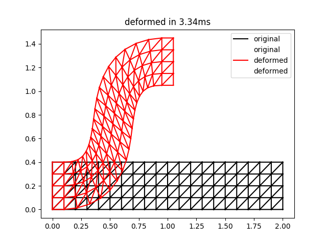
This is qualitatively quite close to the result for two iterations in Figure 3 of the ARAP paper. Note that the timings may be a bit unreliable for such a small problem size.
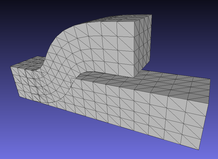
A corresponding result for 3D deformations is here (note that this corrects an earlier bug in rotation computations for 3D):
Performance
By using SciPy's sparse matrix functions and pre-factoring the systems, the solves are very quick. This is because SciPy uses optimized libraries for the factorization and backsolves. Prefactoring the system matrices for efficiency was a key point of the paper and it's nice to be able to take advantage of this from Python.
To look at the breakdown of time taken for right-hand-side computation and solves, I increased the problem size to 100x25, corresponding to a 2500 vertex mesh. Total time for two iterations was roughly 35ms, of which 5ms were the linear solves and 30ms were the right-hand-side computations. So the right-hand-side computation completely dominates the overall time. That said, using a looping approach, I could not even build the Laplace matrix in 30ms to say nothing of building the right-hand-side three times over, so the vectorization has paid off. More profiling would be needed to say if the most time-consuming portion is the SVDs or the indexing but overall I consider it a success to implement a graphics paper that has been cited more than 700 times in 99 lines of Python.